


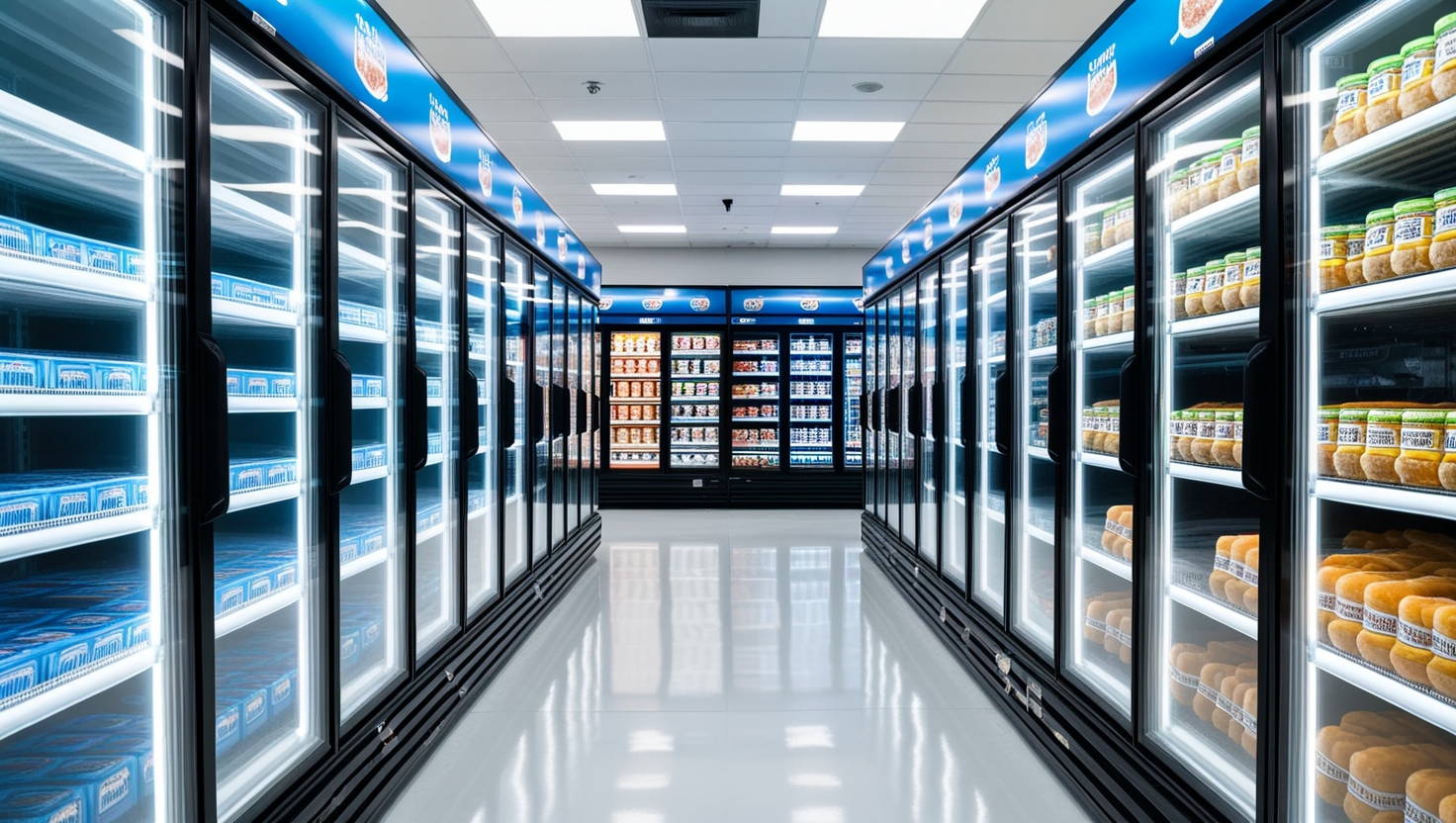
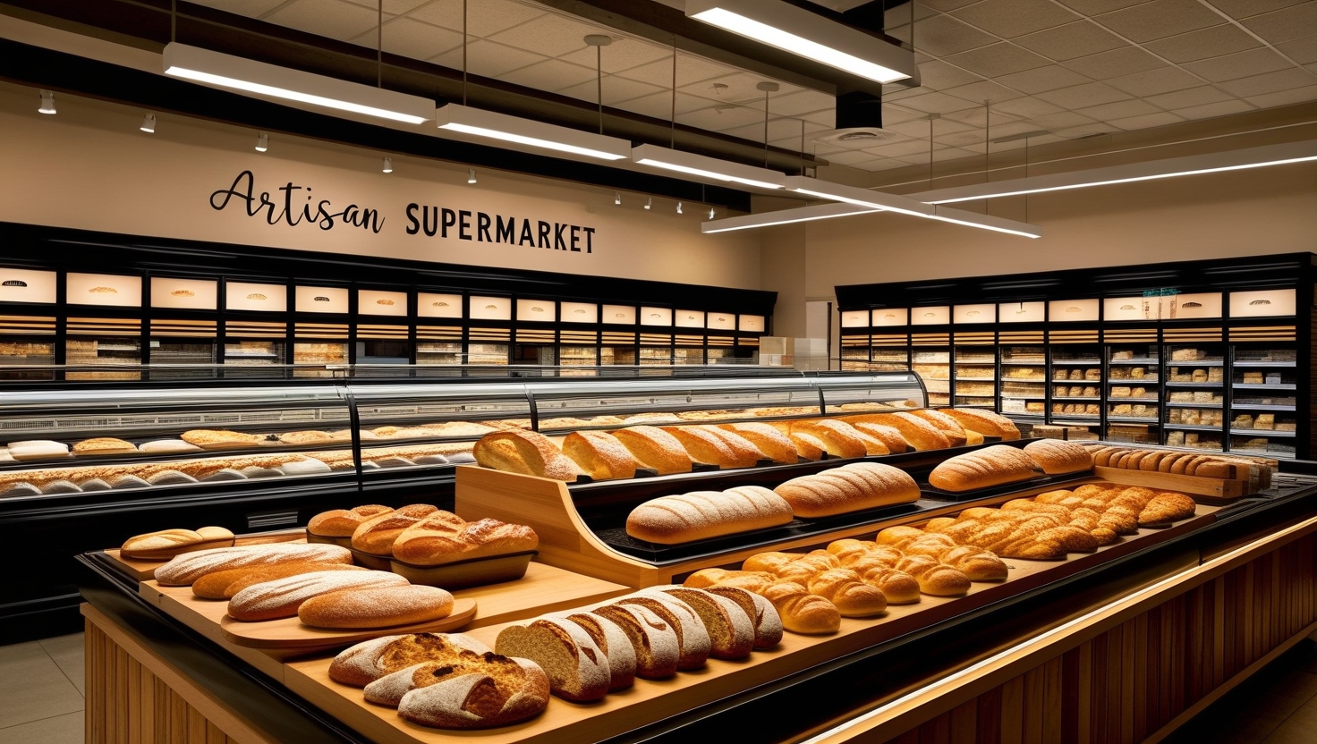
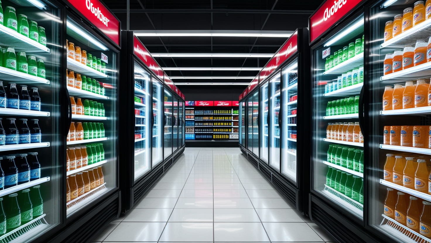
How AI Transforms Food Retail
The evolution from manual to fully autonomous energy management

Phase 1: Rule-Based Automation
Static schedules and simple thresholds - the starting point
Fixed Schedules
Cooling systems run on predetermined schedules (e.g., compressors at 100% from 6am-10pm). No consideration of actual temperature or energy prices.
Simple Thresholds
Temperature-only control: If freezer > -16°C, turn on. If < -20°C, turn off. No optimization between these limits.
Manual Decisions
Store managers manually adjust HVAC settings. No real-time market data integration. Decisions based on "feel" not data.
No BESS Integration
If battery storage exists, it's used only for backup power. No arbitrage trading, no load shifting, no revenue generation.

Phase 2: Predictive AI
ML models predict prices 24h ahead - first arbitrage opportunities
Price Forecasting
ML models (LSTM, XGBoost) predict day-ahead prices with 85% accuracy. System knows when negative prices are coming 24h in advance.
Pre-Cooling Strategy
When negative prices predicted: Pre-cool freezers to -22°C (instead of -18°C). Use thermal mass as free energy storage.
BESS Charging Optimization
Battery charges during predicted low/negative prices, discharges during peaks. Semi-automatic: human approves trading schedule daily.
Weather Integration
Open-Meteo API provides 3-day forecasts. Hot days (+30°C) = pre-cool at night. Cold days = reduce heating during solar peak.

Phase 3: Agentic AI
AI agents trade autonomously - every freezer becomes an edge device
Autonomous Trading Agents
AI agents execute trades without human approval. Real-time intraday market participation. Sub-second decision making.
Edge Computing
Each freezer has local AI chip. Decisions made at device level. Network latency eliminated. Works offline if needed.
Dynamic Load Shaping
System creates artificial "demand valleys" to maximize solar self-consumption. Loads shifted in real-time based on generation.
Predictive Maintenance
AI detects compressor degradation before failure. Scheduled maintenance during low-price windows. Zero unplanned downtime.

Phase 4: Swarm Intelligence
500+ stores act as collective intelligence - Virtual Power Plant
Virtual Power Plant (VPP)
500 stores × 500kWh BESS = 250 MWh storage. 500 stores × 200kW flex load = 100 MW flexibility. Grid-scale market participant.
Collective Optimization
Stores coordinate via federated learning. If Store A has surplus solar, Store B delays its BESS charging. Network-wide efficiency.
Grid Stabilization Services
VPP provides frequency regulation to grid operators. Revenue for helping stabilize renewable-heavy grids.
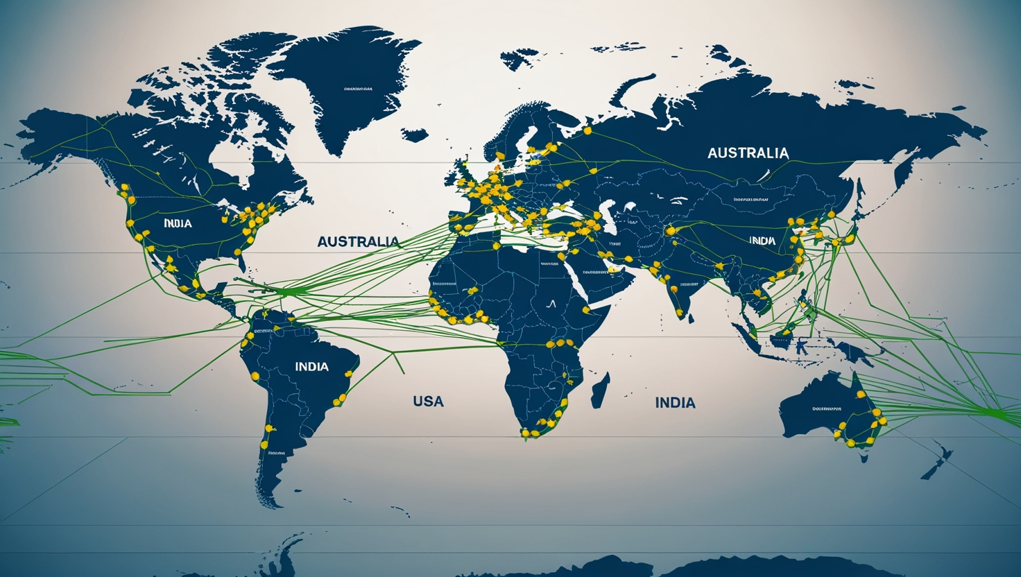
Cross-Border Trading
Australian stores trade with Asian markets. European stores optimize across 27 countries. 24/7 global arbitrage.
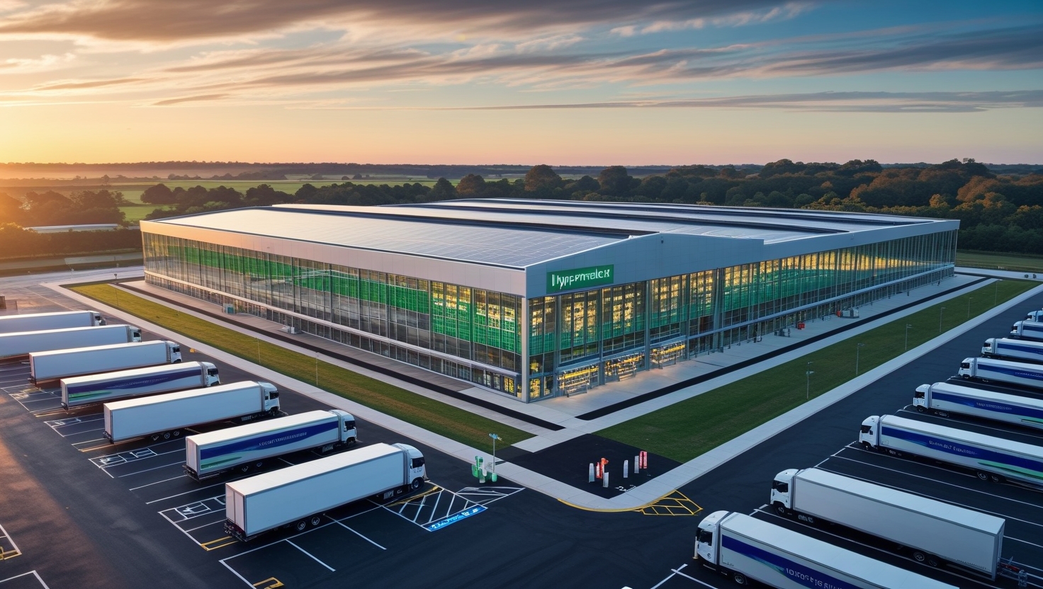
MEGA XXL Store - AI Digital Twin
Interactive visualization of a 10,000m² hypermarket with 2.5 MW load
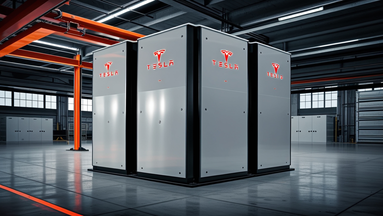
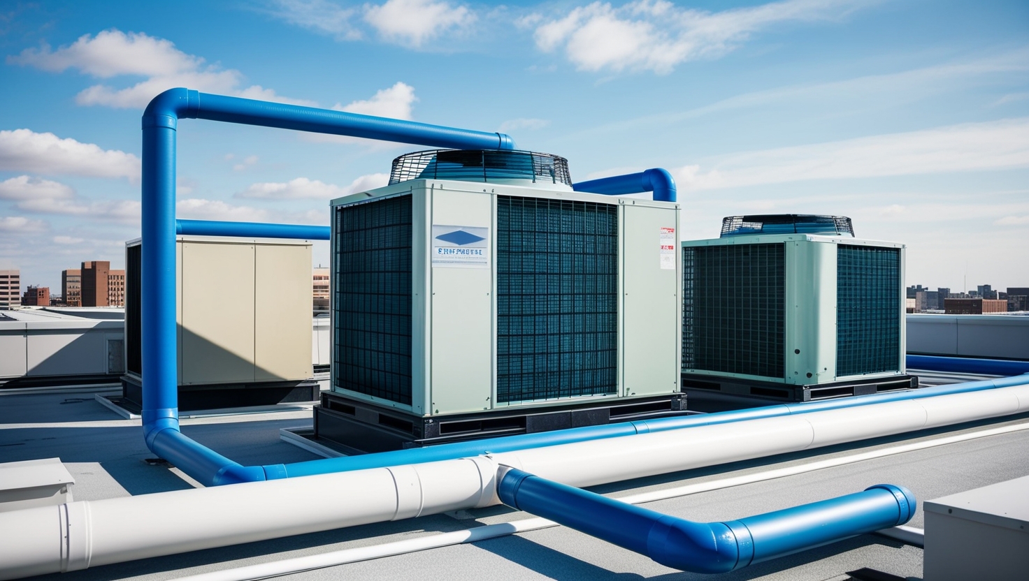
Energy Systems


Store Zones

Weather Impact & Logistics
Real-time weather data drives AI decisions for cooling, heating, and fleet management
 Current Conditions

 Cooling Load Impact

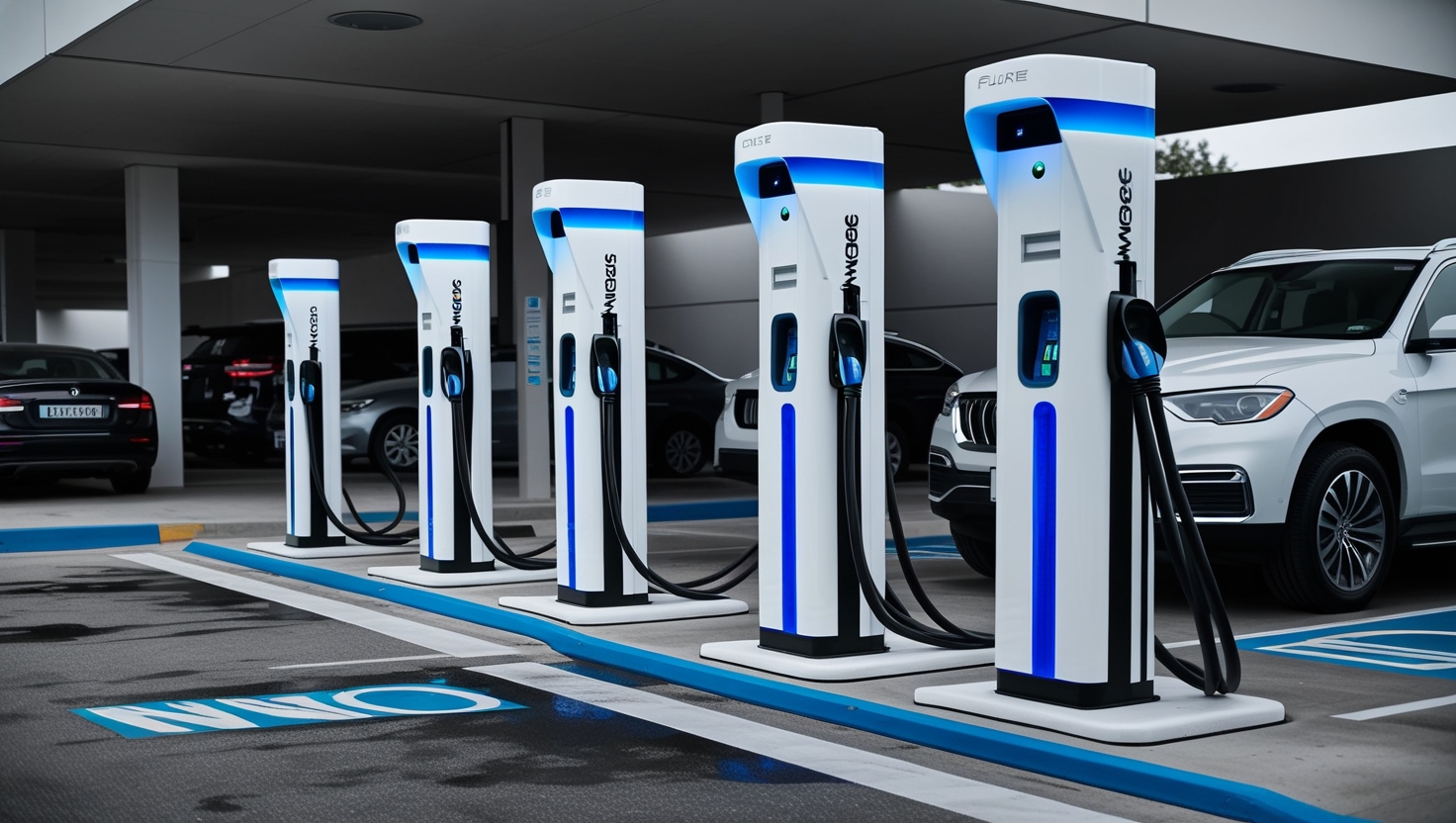
 Electric Fleet Status

 Distribution Centers
Simulation Controls
Adjust parameters and observe the effects on savings and performance
Load Profile vs. Spot Price (24h)
BESS State of Charge & Actions
Cumulative Savings
Cold Chain Temperatures
Simulation Results
Based on AU_SA market data with current settings

Stromfee.AI Academy - Food Retail Module
Learn step by step how to optimize supermarket energy systems
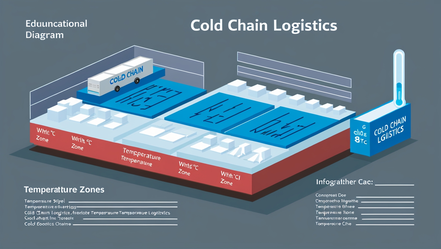
Lektion 1: Cold Chain Basics
Understanding thermal mass, temperature buffers and flexible loads
Lernziele
- Verstehen, wie thermische Masse als Energiespeicher funktioniert
- Temperaturpuffer und ihre Grenzen kennenlernen
- Flexible vs. kritische Lasten unterscheiden
Thermische Masse
Gefrorene Waren speichern Kälte. Ein -18°C Freezer kann auf -22°C vorgekühlt werden = kostenlose Speicherung.
Temperaturpuffer
HACCP erlaubt -18°C bis -15°C. Diese 3°C = 2-4 Stunden Autonomie ohne Kompressor.
Flexible Lasten
Kühlung = 60% des Stromverbrauchs. Davon sind 40% flexibel verschiebbar für Arbitrage.

Lektion 2: Spot Market Trading
Using day-ahead and intraday markets for food retail
Lernziele
- Day-Ahead vs. Intraday Markt verstehen
- Preisspreads identifizieren und nutzen
- Negative Preise als Chance erkennen
Day-Ahead Markt
Handel 12-36h vor Lieferung. Preise bekannt um 12:00 für nächsten Tag. Planungssicherheit.
Intraday Trading
Handel bis 5 min vor Lieferung. Höhere Volatilität = höhere Gewinne bei schneller Reaktion.
Negative Preise
AU_SA: 864h negative Preise/Jahr. Verbraucher werden BEZAHLT um Strom abzunehmen!
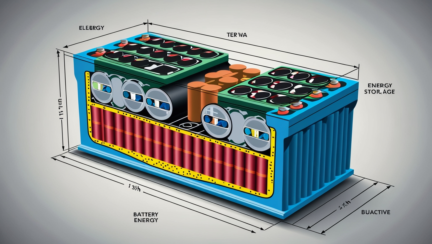
Lektion 3: BESS Sizing for Supermarkets
Calculate optimal storage size based on load profile
Lernziele
- Optimale BESS-Kapazität berechnen
- C-Rate und Zyklen verstehen
- ROI-Berechnung durchführen
Kapazitätsformel
BESS kWh = Peaklast × 2h. Für 2.5 MW Store: 5 MWh BESS als Startwert.
C-Rate Auswahl
C/2 (2h Entladung) für Arbitrage optimal. C/1 für Peakshaving. C/4 für Backup.
ROI Berechnung
Investment: €400/kWh. Revenue: €150/kWh/Jahr bei €500 Spread. Payback: 2.7 Jahre.

Lektion 4: AI-Powered Optimization
Using machine learning for price and load predictions
Lernziele
- ML-Modelle für Preisprognose verstehen
- Lastprognose mit historischen Daten
- Reinforcement Learning für Trading
Preisprognose
LSTM/XGBoost: 85% Accuracy für 24h. Input: Wetter, Solar, Wind, historische Preise.
Lastprognose
Supermarkt-Last vorhersagen: Wochentag, Feiertage, Wetter, Sonderaktionen.
RL Trading Agent
Agent lernt optimale Charge/Discharge-Strategie. Belohnung: €/kWh Spread maximieren.

Lektion 5: Multi-Site Portfolio
Orchestrating 500+ stores as a Virtual Power Plant
Lernziele
- VPP-Architektur verstehen
- Regelenergie-Märkte erschließen
- Federated Learning für Schwarm-Optimierung
VPP Aggregation
500 Stores × 500kWh = 250 MWh. Mindestgröße für FCR-Markt: 1 MW (erreicht mit 5 Stores).
Regelenergie
FCR: €15/MW/h. aFRR: €5-50/MW/h. Supermarkt-VPP kann alle Märkte bedienen.
Swarm Intelligence
Stores teilen Lernfortschritte ohne Daten zu teilen. Datenschutz + kollektive Optimierung.
Lektion 6: Case Study: AU vs US vs IN
Developing market-specific strategies for three continents
Lernziele
- Marktspezifische Strategien entwickeln
- Regulatorische Unterschiede verstehen
- ROI für jeden Markt berechnen
Australien (AU_SA)
€867 Spread, 864 neg. Stunden. Strategie: Aggressive Mittagsladung, Abendentladung. ROI: 1.8 Jahre.
USA (CAISO)
Duck Curve: Tiefpreise 10-15h, Peak 18-21h. Strategie: Solar-Matching + Evening Arbitrage. ROI: 2.5 Jahre.
Indien (IEX)
Morgen+Abend Peaks. Keine neg. Preise. Strategie: Peakshaving + UPS-Funktion. ROI: 3.5 Jahre.
Ready to Transform Your Retail Chain?
Our AI experts will analyze your specific portfolio and calculate your savings potential based on real market data.